Predictive Maintenance: Why I Fell Down the Rabbit Hole
Part 1 of a series on predictive maintenance and anomaly detection
I have wanted to write this series for a long time, and here is the first piece.
Why this series
At university, I meet system identification and estimation as theory: equations, proofs and toolbox commands. It is easy to pass an exam and still not feel how any of it works on a real machine. This series is my attempt to close that gap. I document what I learn as I go, and for each concept I follow one real-life example, such as a thermostat, from the idea to the code to a working fault detector. I write for people who are new to the topic, because not long ago that was me.
A bit about me
I am an engineering student specializing in data science and data engineering, with a focus on System Identification & Data Analysis and Adaptive Learning, Estimation & Supervision.
How I got here
It all started with trains. I wondered how complicated it must be to perform maintenance on trains. While doing some research, I read an article explaining how sensors are placed on trains to collect data. This data is then analyzed and used for forecasting, to predict when maintenance will be needed. By doing this, operators were cutting costs significantly.
That was my introduction to predictive maintenance and anomaly detection, and I found it interesting enough to pursue a postgraduate degree in the field.
What this series covers
System identification means building a mathematical model of a system from its input and output data. There are three approaches:
- White box: you know the physics and write the equations directly.
- Grey box: you know part of the physics, and data fills in the rest.
- Black box: you do not model the internals at all. You let the data describe the behavior.
This series focuses on black box, data-driven models. We will start with the simplest kind: SISO (single-input, single-output) models, which look at one signal at a time, such as the temperature reading from your house thermostat.
AR, MA and ARIMA
In this part, we will look at three models. They all predict the next value of a signal from its own history.
AR (AutoRegressive). The next value depends on the previous values of the signal itself:
\[ y(t) = \theta_1\, y(t-1) + \theta_2\, y(t-2) + \dots + \theta_p\, y(t-p) + e(t) \tag{1}\]
where:
- \(y(t)\): the value of the signal now, for example the thermostat temperature at the current time step \(t\).
- \(y(t-1)\): the value one time step ago, meaning the previous measurement. In the same way, \(y(t-2)\) is two steps ago, and so on.
- \(\theta_1, \dots, \theta_p\): weights that the model learns from data. Each one says how much the matching past value matters for predicting the next one.
- \(p\): how many past values the model looks back at.
- \(e(t)\): the error (or noise) term. It is the part of the current value that the past values cannot explain: random, unpredictable, and zero on average. In engineering it is called white noise.
Think of your thermostat reading. The room temperature changes slowly, so where it is now tells you where it will be a few minutes from now.
MA (Moving Average). The next value depends on past prediction errors (the “shocks” the model did not see coming):
\[ y(t) = e(t) + c_1\, e(t-1) + c_2\, e(t-2) + \dots + c_q\, e(t-q) \tag{2}\]
where:
- \(e(t)\): the error at the current time step, the new random shock that has just hit the system.
- \(e(t-1)\): the error one step ago, the shock from the previous time step. \(e(t-2)\) is the one before that, and so on.
- \(c_1, \dots, c_q\): weights the model learns. Each says how much of an earlier shock is still affecting the signal.
- \(q\): how many past errors the model remembers.
(I use \(c\) for these weights so they are not confused with the \(\theta\) weights of the AR model.)
Imagine someone opens a window. The temperature dips, then recovers over the next few minutes. That short-lived disturbance is what MA captures.
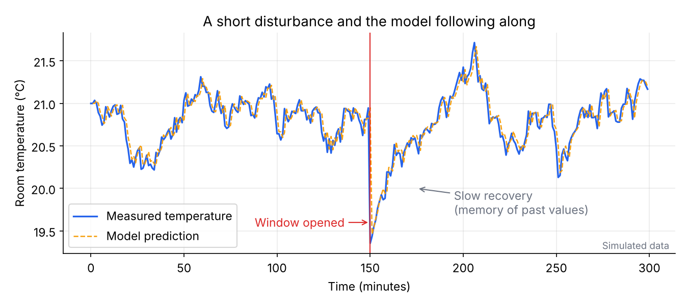
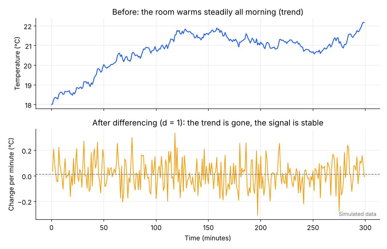
ARIMA. AR and MA combined, with an added step called integration (I). Many real signals trend upward or downward over time, like the room warming up all morning as the sun comes in. ARIMA handles this by modeling the change between samples (differencing) instead of the raw values:
\[ \nabla y(t) = y(t) - y(t-1) \tag{3}\]
The model is written \(\mathrm{ARIMA}(p, d, q)\), where:
- \(p\): how many past values to use (AR order)
- \(d\): how many times to difference the data
- \(q\): how many past errors to use (MA order)
Why this matters for anomaly detection
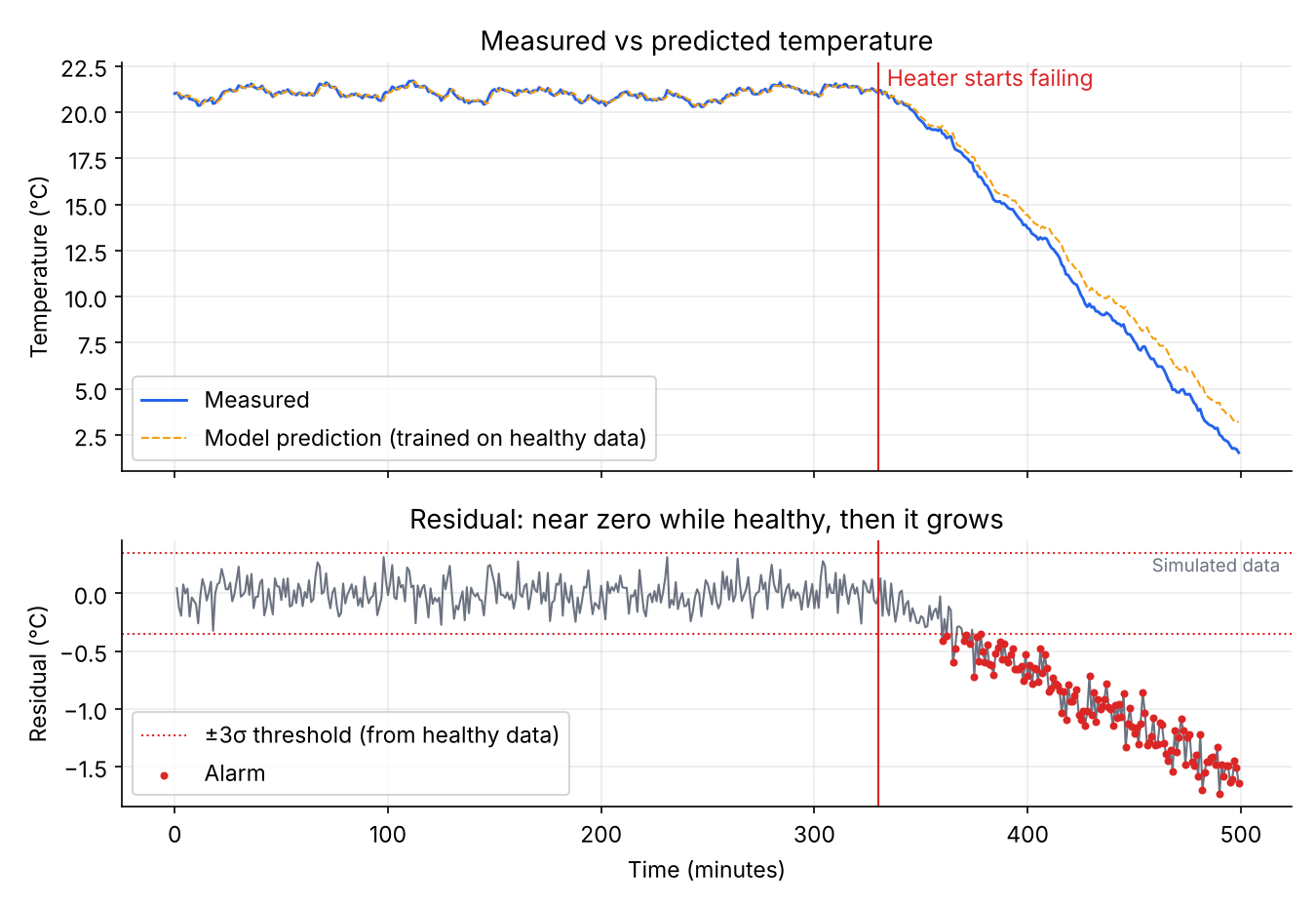
Here is the idea that ties it all together. Train a model on healthy data. Then, as new data comes in, compare the model’s prediction \(\hat{y}(t)\) with what the sensor actually reports, \(y(t)\). The difference is the residual:
\[ r(t) = y(t) - \hat{y}(t) \tag{4}\]
While the machine is healthy, the residual stays small. When something starts to go wrong, the residual grows, and that is your early warning.
For the thermostat: if the heating is working normally, the model predicts the temperature well. If the heater starts failing, the real temperature keeps falling below what the model expects, and the residual grows.
Conclusion
To sum up: AR models the memory of a signal, how its past values shape the next one. MA models disturbances, the short-lived shocks that a healthy system experiences, like an open window. ARIMA combines both and also removes trends through differencing.
An important point is that the disturbances MA captures are normal, not faults. A fault only shows up when the residual becomes much larger than these normal shocks. All of this relies on past data, and that data must come from a healthy system, so the model learns what normal looks like.
Next time
In Part 2, we will look at how to choose the model’s parameters and check that it is good enough. In Part 3, we will use it to catch a fault in Python.