Predictive Maintenance: Choosing and Checking a Model

Part 2 of a series on predictive maintenance and anomaly detection

How to choose p, d and q, and how to check that an ARMA model is good enough, using a thermostat example and Python.

In Part 1 we met three models: AR, MA and ARIMA. We also saw the main idea behind anomaly detection: train a model on healthy data, then watch the residual. Before we can do that, we need a model we can trust. In this part we answer two questions:

1. How do I choose the model’s parameters \(p\), \(d\) and \(q\)?
2. How do I know the model is good enough?

In Part 3 we will use the model to catch a fault.

The data

I use the thermostat example again, with simulated data so that we know what is really going on. The room temperature is recorded once per minute. For the first 400 minutes the heating is healthy, and this is the only part we use in this post. (The heater starts to fail after minute 400, but that is the story of Part 3.)

The healthy data comes from an ARMA(2,1) process around 21 °C. That means a “right answer” exists, but we will pretend we don’t know it, as in real life. The full script is in part2_choose_check_model.py, and you can run it yourself.

The rule for everything below: the model is fitted on healthy data only.

Step 1: choose d

What “stationary” means

Picture a dog on a leash walking around its owner. It wanders, but it never goes far, and the size of its wandering stays about the same. That is a stationary signal. The thermostat is like this: the room temperature wiggles around 21 °C, and both the average and the size of the wiggles stay the same hour after hour.

Now picture the dog walking away down the road. It has no “home” position, so the average keeps moving. That is a non-stationary signal. A room that warms up all morning as the sun comes in is like this.

AR and MA models learn a fixed recipe (the weights \(\theta\) and \(c\)) from past data. That recipe only works if the signal behaves the same way all the time. If the average keeps drifting, a recipe learned on the first hour does not fit the next hour.

Figure 1: Left: a stationary signal stays around a fixed level. Middle: a trending signal drifts away. Right: the trending signal after differencing is stable again (simulated data).

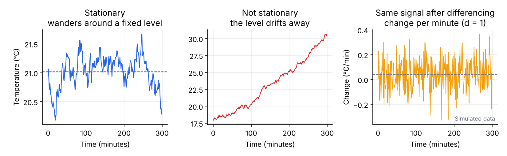
Differencing: model the change, not the level

If a signal trends, we stop modeling the temperature itself and model how much it changed each minute instead:

Minute	Temperature	Change from the minute before
1	18.0
2	18.3	+0.3
3	18.7	+0.4
4	19.0	+0.3
5	19.4	+0.4

The temperature climbs steadily, but the changes stay around +0.35, which is stable. We removed the trend, as in the right-hand plot of Figure 1. That is d = 1: we differenced once. d = 2 means we differenced the changes again, which is only needed if the change itself keeps trending. Use no more differencing than necessary, because each round adds noise. In practice \(d\) is almost always 0, 1 or 2.

The ADF test: a statistical check

A plot is not always enough, so we use a test. The Augmented Dickey-Fuller (ADF) test begins by assuming the signal is not stationary, meaning it has no tendency to return to an average. It then asks: if that were true, how likely is it that I would see data that keeps coming back to its average like this? That probability is the p-value.

• Small p-value (below 0.05): such data would be very unlikely under the “not stationary” assumption, so we reject it. The signal is stationary and d = 0.
• Large p-value (above 0.05): we cannot rule out non-stationarity. Difference once (\(d = 1\)), then test again.

from statsmodels.tsa.stattools import adfuller

adf_p = adfuller(y_healthy)[1]     # [1] picks the p-value; p < 0.05 -> stationary

For our healthy data the p-value is below 0.05, so the signal is stationary and d = 0. A thermostat holds the room around a set value, so this is what we expect.

Be careful not to mix this up with the Ljung-Box test in Step 4, which reads the other way around:

Test	Good result	Meaning
ADF	small p-value	the signal is stationary
Ljung-Box	large p-value	the residuals are white noise

Step 2: get a first guess for p and q

Two plots give a starting point.

The ACF (autocorrelation function) asks: how much does the signal resemble its own past? Take the temperature series, shift a copy of it by one minute and measure how similar the two are. That is the correlation at lag 1. Do the same with a five-minute shift for lag 5, and so on. Values run from −1 to 1, and 1 means identical behavior. For our thermostat, lag 1 is about 0.93: the temperature now is very similar to a minute ago. The bars shrink as the lag grows, because the room gradually forgets. That slow fading is the memory of the system.

The PACF (partial autocorrelation function) fixes a flaw of the ACF. The temperature 3 minutes ago seems related to the temperature now, but partly only because both are related to the minutes in between. It is like gossip: A tells B, and B tells C. A and C look connected, but once you know B, A adds nothing. The PACF removes these indirect links. At each lag it asks: once I already know the more recent values, does this older value tell me anything new?

Figure 2: ACF and PACF of the healthy thermostat data. The shaded band is the 95% confidence range: bars inside it are not significantly different from zero (simulated data).

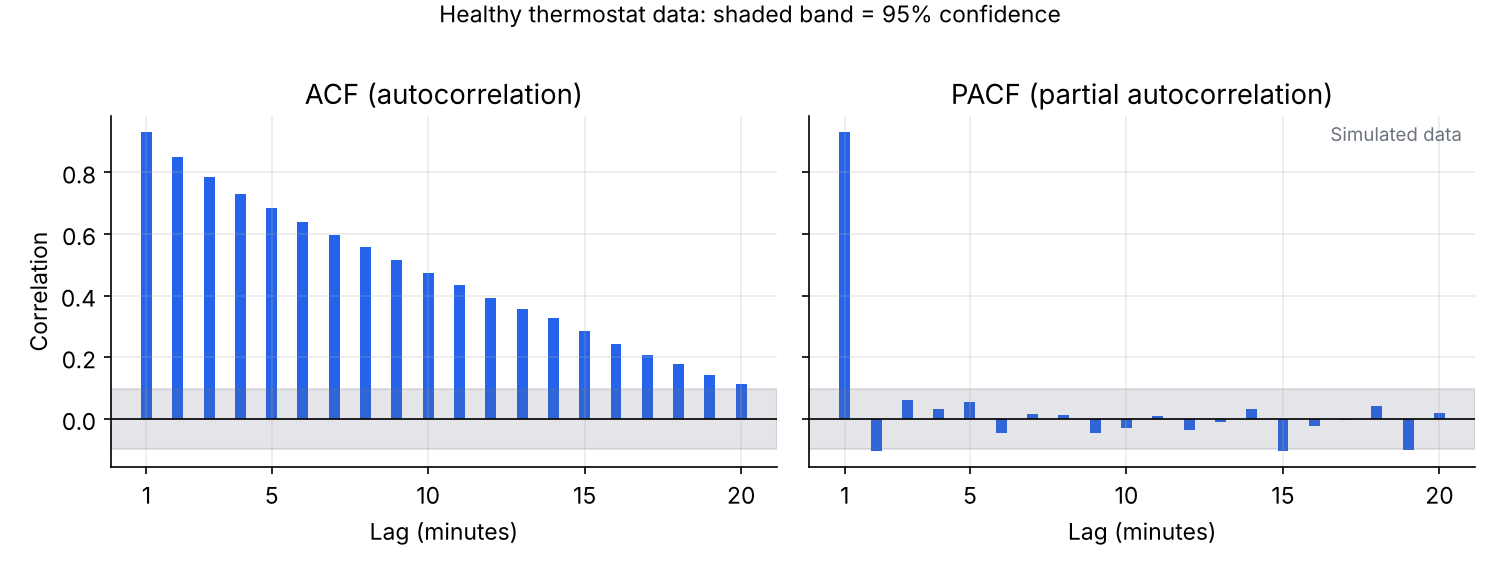
The shaded band marks the range where a bar could be just random chance, so bars inside it count as zero. Use these rules to read the plots:

What you see	It suggests
PACF cuts off after lag \(p\), ACF decays slowly	AR(\(p\))
ACF cuts off after lag \(q\), PACF decays slowly	MA(\(q\))
Both decay	a mix, so let AIC and BIC decide

In Figure 2 the ACF decays slowly, and the PACF has one clear spike at lag 1, then falls inside the band. Once you know last minute’s temperature, older minutes add nothing new, so this points to \(p = 1\). It is only a guess, and real data is rarely this clean, so in the next step we let the numbers compare candidates.

Step 3: compare models with AIC and BIC

A bigger model always fits the training data better, but it may just be memorizing noise. AIC and BIC reward a good fit and penalize complexity:

\[ \mathrm{AIC} = 2k - 2\ln \hat{L} \tag{1}\]

\[ \mathrm{BIC} = k\ln n - 2\ln \hat{L} \tag{2}\]

Here \(k\) is the number of parameters (the AR weights, the MA weights, the mean and the noise variance), \(n\) the number of samples, and \(\hat{L}\) the best likelihood the model reaches. Lower is better. BIC punishes extra parameters more, so it tends to pick simpler models.

We fit every combination of \(p\) and \(q\) from 0 to 3:

from statsmodels.tsa.arima.model import ARIMA

for p in range(4):
    for q in range(4):
        res = ARIMA(y_healthy, order=(p, 0, q), trend="c").fit()
        print(p, q, res.aic, res.bic)

Here are some of the results, together with the Ljung-Box check from the next step:

Model	\(k\)	AIC	BIC	Ljung-Box p
MA(2)	4	−451.0	−435.0	< 0.001
AR(1)	3	−696.8	−684.9	0.363
AR(2)	4	−699.5	−683.5	0.701
ARMA(1,1)	4	−700.1	−684.1	0.754
ARMA(2,1)	5	−699.0	−679.1	0.781
ARMA(3,3)	8	−697.3	−665.4	0.422

Your numbers may differ in the last digits.

Three things stand out:

• MA(2) is far behind. It has no memory of past values, which this signal clearly needs.
• The next four are almost tied. A difference of less than about 2 points is usually not meaningful.
• The big ARMA(3,3) does not win. More parameters did not buy a better model, and the penalty shows.

AIC picks ARMA(1,1) and BIC picks the simpler AR(1). When they disagree, AIC favors prediction accuracy and BIC favors simplicity. Our goal is good predictions, because the residual is what we monitor, so I go with ARMA(1,1). AR(1) would also be a reasonable choice.

Step 4: is the model good enough?

AIC and BIC pick the best among the candidates, but they cannot tell you whether the winner is actually good. For that, look at the residuals. If the model captured every real pattern, what is left should be white noise: random, with no structure left to learn.

The Ljung-Box test checks this with one number. Its starting assumption is that the residuals are white. It adds up the squared autocorrelations \(\hat\rho_k\) of the residuals up to lag \(h\):

\[ Q = n(n+2)\sum_{k=1}^{h}\frac{\hat\rho_k^{\,2}}{n-k} \tag{3}\]

and compares \(Q\) with a \(\chi^2\) distribution with \(h-(p+q)\) degrees of freedom.

from statsmodels.stats.diagnostic import acorr_ljungbox

acorr_ljungbox(res.resid[5:], lags=[10], model_df=p + q)

• p-value above 0.05: no leftover pattern. The model is good enough.
• p-value below 0.05: structure remains, so the model is too simple (underfitted). Try a higher \(p\) or \(q\), recheck \(d\), or add a seasonal component if the pattern repeats daily.

Figure 3: Autocorrelation of the residuals. Left: a model that is too simple leaves strong structure behind. Right: the chosen ARMA(1,1) leaves only noise (simulated data).

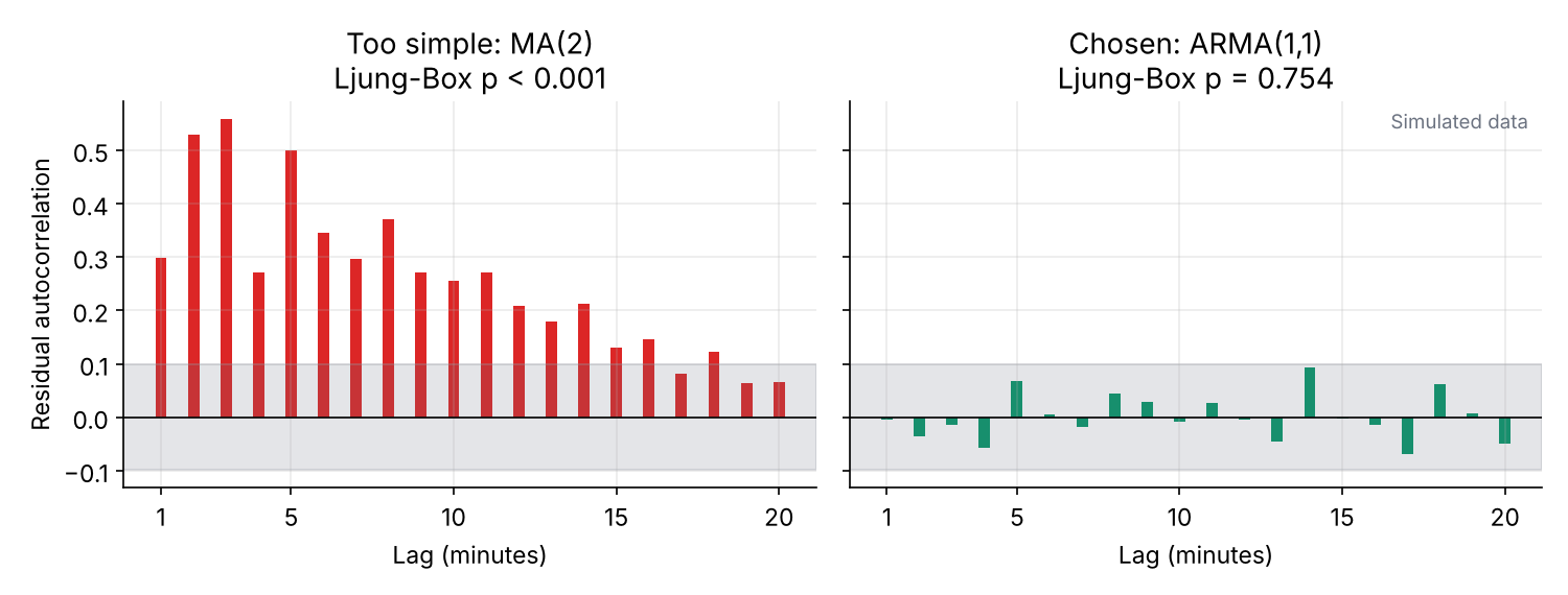
Figure 3 shows the difference. The workflow is: AIC and BIC choose the winner, Ljung-Box confirms it.

Our final model, fitted on the healthy data, is:

\[ y(t) - 21.01 = 0.911\,\big(y(t-1) - 21.01\big) + e(t) + 0.130\, e(t-1) \tag{4}\]

The number 21.01 is the mean temperature. The weight 0.911 says the room has a long memory: this minute’s temperature is mostly last minute’s, which is the thermal inertia we talked about in Part 1. The weight 0.130 on the previous error is small. In the statsmodels output these appear as const, ar.L1 and ma.L1, which correspond to the mean, \(\theta_1\) and \(c_1\) in the notation of Part 1. The typical size of the residual is \(\sigma \approx 0.10\) °C. We will use this model in Part 3.

Conclusion

The workflow for choosing and checking a model of a single signal:

1. Check stationarity (ADF) and pick \(d\).
2. Look at ACF and PACF for a first guess of \(p\) and \(q\).
3. Fit candidates on healthy data and compare AIC and BIC.
4. Confirm with Ljung-Box that the residuals are white.

Every step uses healthy data to learn what normal looks like. Once the model passes these checks, we can trust its predictions, and anything it cannot explain is worth a closer look.

Next time

In Part 3, we apply this model to new data from the thermostat, where the heater slowly starts to fail, and use the residual to raise an alarm.