Predictive Maintenance: Catching the Fault

Part 3 of a series on predictive maintenance and anomaly detection

How to turn a model’s residuals into an alarm, using a threshold and a CUSUM, with a thermostat example and Python.

In Part 2 we chose and checked a model of the room temperature, using only healthy data. In this part we put it to work: we use it to notice that the heater is failing, from the temperature alone.

Where we left off

All you need from Part 2 is this. We fitted an ARMA(1,1) model to 400 minutes of healthy thermostat data:

\[ y(t) - 21.01 = 0.911\,\big(y(t-1) - 21.01\big) + e(t) + 0.130\, e(t-1) \tag{1}\]

It predicts each minute’s temperature from the previous minutes, and the typical size of its error while the room is healthy is \(\sigma \approx 0.10\) °C. In statsmodels:

from statsmodels.tsa.arima.model import ARIMA

model = ARIMA(y_healthy, order=(1, 0, 1), trend="c").fit()

The full script is in part3_catch_fault.py.

The scenario

The data is simulated again, once per minute. For the first 400 minutes the heating is healthy. After that the heater starts to fail: a heating shortfall that grows a little every minute. The model has never seen this part of the data.

The idea is simple. While the room is healthy, the model’s guesses are close to the real temperature. Once the heater fails, the real temperature falls below the guesses, and the gap between them (the residual) keeps growing. We turn that gap into an alarm.

Step 1: measure the gap

We apply the same fixed model to all the data, healthy and faulty, without refitting it. For each minute the model makes a guess, and the residual is how far the real temperature is from that guess:

\[ r(t) = y(t) - \hat{y}(t) \]

full = model.apply(y)                  # same parameters, new data
resid = full.resid
sigma = resid[5:400].std()             # typical size of the error while healthy
z = resid / sigma                      # residual measured in "sigmas"

The number \(\sigma\) is the typical size of the model’s error while everything is healthy, here about 0.10 °C. Dividing by it gives \(z\), which says how many typical errors the current error is. A value of \(z = 0.5\) is an ordinary wobble, and \(z = -4\) is very unusual. This puts every residual on the same scale, whatever the sensor measures.

Step 2: a simple alarm, the ±3σ threshold

The simplest alarm is a threshold: raise it when the residual goes beyond \(\pm 3\sigma\), meaning \(|z| > 3\). If the noise is normally distributed, only about 1 point in 370 crosses this line by chance, so a crossing is a good sign that something has changed.

Its weakness is that it reacts to single points. A single spike can give a false alarm, and a slow drift that stays just inside the line can go unnoticed for a long time.

Step 3: CUSUM, the alarm that remembers

The CUSUM (cumulative sum) fixes this by adding up small but persistent errors, like a bucket that slowly fills with water. Since a failing heater makes the temperature fall, we watch for downward shifts:

\[ S(t) = \max\big(0,\; S(t-1) - z(t) - k\big) \tag{2}\]

In words: take the previous total \(S(t-1)\) and add the new drop \(-z(t)\). Subtract a small allowance \(k\) and never let the total go below zero. The constant \(k = 0.5\) means that wobbles within half a sigma are ignored, so while the room is healthy the bucket drains as fast as it fills and \(S\) stays near zero. When the residual keeps falling below zero, the bucket fills steadily. When \(S(t)\) rises above a threshold \(h = 8\), we raise the alarm.

Figure 1: Top: the thermostat signal with the fault starting at minute 400. Middle: the residual measured in sigmas, with the ±3σ threshold. Bottom: the CUSUM, which crosses its threshold at minute 440 (simulated data).

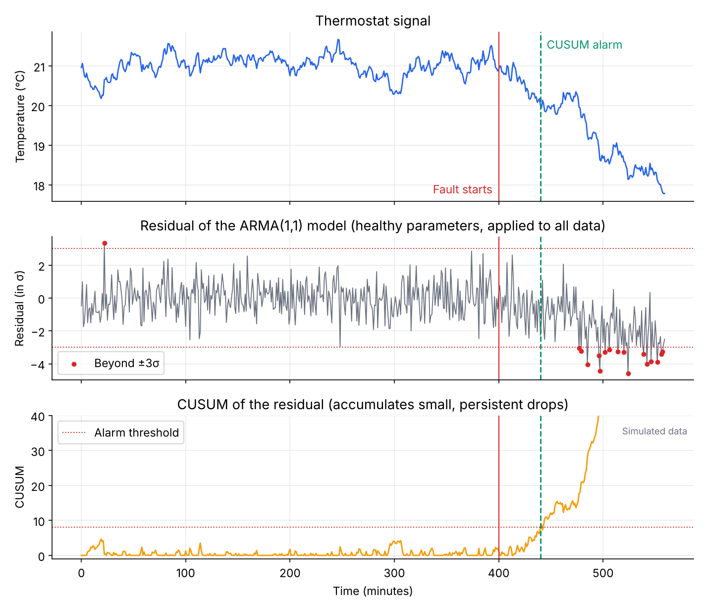
What the figure shows

• During the healthy period the residual looks like noise. The ±3σ rule raised one false alarm at minute 22, a single spike. A few false alarms are expected over hundreds of samples.
• After the fault the residual slowly drifts below zero. The first ±3σ alarm came at minute 477, 77 minutes after the fault began.
• The CUSUM alarmed at minute 440, 40 minutes after the fault began. By then the temperature had fallen from about 20.9 °C to 20.0 °C, a drop you would hardly notice in the room. The model noticed it because it knows how the healthy signal normally behaves.

Is this a lucky run?

To check, I repeated the experiment with 30 different random seeds. A single ±3σ threshold raised at least one false alarm in 21 of the 30 runs. The CUSUM raised none, and detected the fault after a median of about 40 minutes. With \(h = 5\) instead of 8, about half of the runs had false alarms, so thresholds must be tuned on healthy data. You can repeat this check with the robustness() function in the script.

How control systems use this

In control and supervision, the residual is the main signal for fault detection. It goes through three steps:

1. Generate: compare the model’s prediction with the real measurement.
2. Evaluate: is the residual the size we would expect from a healthy machine? (\(\pm 3\sigma\), CUSUM)
3. Decide: raise an alarm, or not.

One catch: a feedback controller can hide a fault by working harder to compensate. A failing heater may keep the room at 21 °C by running at full power. That is why supervision monitors residuals and control effort, not only the output. In our example the thermostat was not compensating, which is why the temperature itself fell.

Conclusion

The workflow for catching a fault:

1. Build and check a model on healthy data (Part 2).
2. Apply the fixed model to new data and compute the residual.
3. Measure the residual in sigmas, using the spread from the healthy period.
4. Watch it with a threshold and a CUSUM, and tune both on healthy data.

A fault is anything the model cannot explain, and the CUSUM notices small drifts that a single threshold misses.

Next time

So far we have looked at one signal at a time. Real machines have many inputs and many outputs, such as heater power, outside temperature and several rooms. In Part 4 we move to MIMO (multiple-input, multiple-output) models.